CCIT4076 Engineering and Information Science

Laboratory 6: Radio Communication

HKU SPACE Community College, Fall 2022

1        Amplitude Modulation of Audio Signals

Suppose a message-carrying signal m(t) is stored in the array m. One may generate the corresponding AM signal s(t) by the built in function ammod as follows:

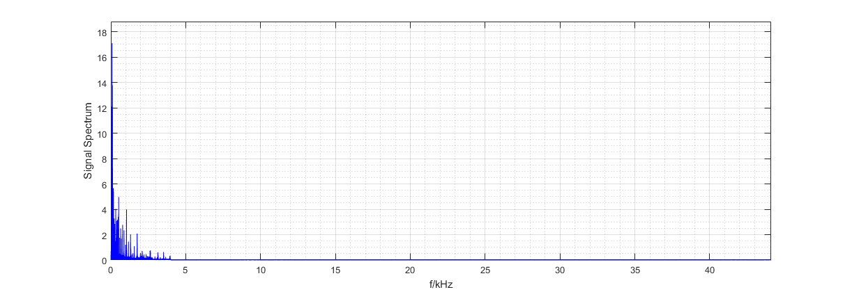
where fc is the target carrier frequency; fs is the sampling frequency (to be loaded together with the message signal array m).  By using the given spectrum visualizer script EIS_spectrum.m, we are allowed to see the following spectra for m(t) and s(t) respectively.

Figure 1: Spectrum of m(t)

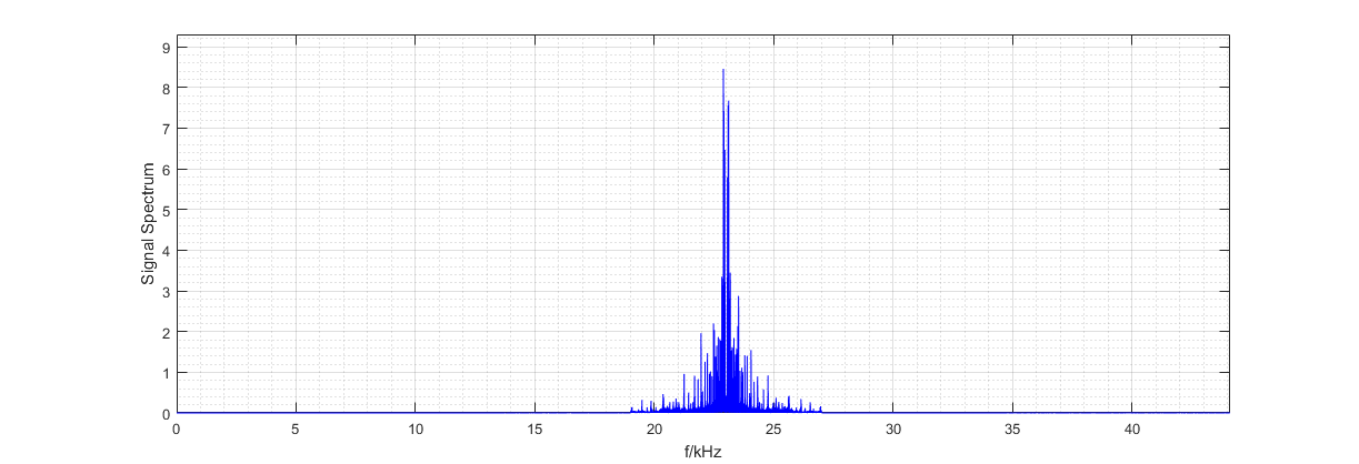
Figure 2: Spectrum of AM-modulated signal s(t).

And if you want to play the AM signal out, you may use the command line sound(s, fs) with no surprise. Because the message is carried to around 23kHz, we are unable to listen to the message audio’s content. In order to migrate it back to an audible range, one may use the demodulation command:

which should look almost exactly the same as in Figure 1. By this point, if you listen to the demodulated signal output v(t) by the command line sound(v, fs), we are allowed to listen to the message audio clearly.

2        Frequency Division Multiplexing

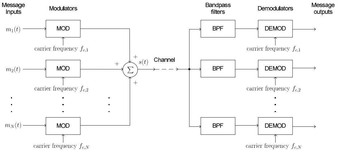
Next, we consider Frequency Division Multiplexing (FDM). The system block diagram is captured as follows:

Figure 3: System Block Diagram of FDM.

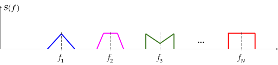
The transmission spectrum of the FDM signal s(t) should look like:

Figure 4: Spectrum of FDM Signal

Precisely, we assign the different channels to different messages to be sent out via the radio spectrum.  The null space (i.e. the unused spectrum) between each channel is referred to as the guardband. As seen from the above block diagram, we need to choose an appropriate BPF before passing S(f) through a demodulator so that co-channel interference is prohibited.

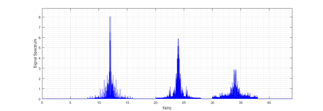
You are given an AM-FDM multiplexed transmission signal in the file radiosignal.wav. Load it onto the workplace and plot the spectrum it using the given spectrum visualizer.

Figure 5: Octave Spectrum Visualization of a given Radio Signal

First, determine the three carrier frequencies used. Then, design three appropriate BPFs to extract the three messages from the given FDM signal by using the flexible filter function EIS_Filter.m. Finally, recover the three message signals respectively. The expected code fragment should look like: